There are exactly three distinct two-dimensional unital algebras over the reals, up to isomorphism. Each of these algebras corresponds to a unique geometry, with applications. This talk will develop the concepts needed to understand two-dimensional algebras over the reals, starting from the definitions of key concepts. We will rediscover the familiar complex numbers and generalize its construction to find the other hypercomplex number systems. We will then prove the result that these are the unique hypercomplex number systems, up to isomorphism. Finally, we will discuss possible generalizations to $n$ dimensions. Please ensure that you have a good understanding of fundamental concepts of two-dimensional linear algebra.

We will use Catoni, F., Cannata, R., Catoni, V., & Zampetti, P. (2004) as a reference.

Outline

• Definition of the complex number field $\mathbf{C}$ (20 mins)

  • Rotation matrices in two dimensions

  • Dilation matrices in two dimensions

  • Proofs and definitions of various facts and operations

  • Geometry of the complex numbers

• Unital algebras (5 mins)

  • Definition of key terms

  • Definition of related concepts

• Discovery of the hypercomplex number systems (20 mins)

  • General $2\times 2$ real matrices

  • The split-complex numbers, and geometry thereof

  • The dual numbers, and geometry thereof

• Applications of the hypercomplex numbers (10 mins)

  • Interval analysis

  • Differentiation of analytic functions

• Equivalence of hypercomplex number algebras up to isomorphism (5 mins)

• Generalizations (5 mins)

  • Potential generalization to $n$ dimensions

Background

The hypercomplex numbers were introduced by Marius Sophus Lie, a Norwegian mathematician. They have applications to geometry, and perhaps more surprisingly, to other fields as well, including calculus.

Our goal in exploring the world of hypercomplex numbers is to:

• understand the complex numbers as an algebra over the reals

• list and understand the basic desirable properties of complex numbers that can be generalized

• find generalizations of complex numbers in two dimensions

• explore the properties, including the geometry, of these generalizations

• explore possible further generalizations

We will use the references listed below for this talk:

• Catoni, F., Cannata, R., Catoni, V., & Zampetti, P. (2004). Two-dimensional hypercomplex numbers and related trigonometries and geometries. Advances in Applied Clifford Algebras, 14(1), 47-68. doi:10.1007/s00006-004-0008-2

The Definition of the Complex Number Field $\mathbf{C}$

For this talk, we will primarily work within $\mathbf{R}^2$. We will first focus our attention on linear transformations of two types: rotations and dilations. A rotation is a distance-preserving transformation that only changes angle, and a dilation is a simple transformation that uniformly scales all distances. In particular, we allow the projection of everything onto the origin to be a dilation, and we allow reflections across the origin also.

We note that all dilations can be expressed as

for $t∈\mathbf{R}$ a free parameter.

We note that all rotations can be expressed as the orthogonal matrices

for $θ∈\mathbf{R}$ a free parameter.

Let a rotation-dilation be a linear transformation that rotates an object, then dilates it. Then all rotation-dilations are of the form

for $t∈\mathbf{R}$ and $θ∈\mathbf{R}$ free parameters.

By making the substitution $a = t\cos θ$ and $b = t\sin θ$, we can express this as

We now have a characterization of all linear transformations that either dilate or rotate the two-dimensional plane. The operation of matrix multiplication represents the composition of these linear transformations. Thus we have defined an algebra which allows us to describe all of these kinds of transformations, and the relationship between them. This algebra of dilations and rotations, as some of you might recognize, has a name. It's the algebra of complex numbers. We define

and for ease of notation, we will denote by $1_\mathbf{C}$ (or simply $1$) the matrix $\begin{bmatrix} 1 & 0 \\ 0 & 1 \end{bmatrix}$, and by $\mathrm{i}$ the matrix $\begin{bmatrix} 0 & -1 \\ 1 & 0 \end{bmatrix}$. Let us investigate some properties of this algebra.

Properties

We inherit certain properties of complex numbers directly from the definition:

• $\mathbf{C}$ is a two-dimensional vector space over $\mathbf{R}$

• multiplication distributes over addition

• multiplication is associative

• there is a multiplicative identity, and it's $1_\mathbf{C}$

• there is an additive identity, and it's $0_\mathbf{C}$

• every element has an additive inverse

It turns out that we can recover the other properties of the complex numbers easily from this definition.

Dilation matrices commute with all other matrices because they are multiples of the identity. And rotation matrices commute with themselves, because the composition of two rotation matrices is simply the addition of angles. So all matrices of the form $tR$ commute with each other. Therefore, $\mathbf{C}$ is a commutative algebra.

Let $z=a1_\mathbf{C}+b\mathrm{i}∈\mathbf{C}$ and define

(note that this is the norm usually used in algebra; the norm used in analysis is the square root) and from the multiplicative property of the determinant, we see that this norm is multiplicative; i.e. if $w∈\mathbf{C}$ and $z∈\mathbf{C}$, then

Let us now define an involution, called the conjugate:

and note the following familiar results:

• $\overline{\overline{z}} = z$

• $\overline{tz + w} = t\overline{z} + \overline{w}$

• $\overline{zw} = \overline{w}\overline{z} = \overline{z}\overline{w}$

• $\|\overline{z}\| = \|z\|$

inherited from known properties of the transpose. We can also note there is a natural embedding of the real numbers within this complex field; they correspond to exactly the self-conjugate complex numbers; i.e. the symmetric matrices.

Note that, if $z = a1_\mathbf{C} + b\mathrm{i}$, then

which, interestingly, means that if $a^2 + b^2 \ne 0$, then

so if $z \ne 0_\mathbf{C}$, then there is $z^{-1}$, an inverse for $z$. We have, here, verified all the field axioms (in a somewhat disorganized fashion). So $\mathbf{C}$ is a field.

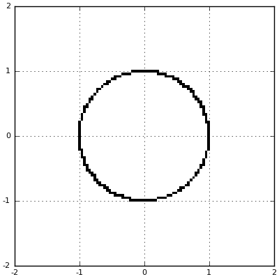
You may already be familiar with the geometry of complex numbers. After all, it's the standard Euclidean geometry that we see every day. The unit circle on the complex numbers is the familiar unit circle:

Unital Algebra

Let us define formally an algebra $A$ over a field $\mathbf{R}$ as a vector space $A$ over $\mathbf{R}$ with an additional bilinear binary operation, multiplication $A × A \to A$. The requirement that the operation is bilinear can be restated as:

We require that this binary operation is compatible with the scalar multiplication; that is, if $s∈\mathbf{R}$, $t∈\mathbf{R}$ and $x∈A$, $y∈A$, then $(sx)(ty) = (st)(xy)$.

We also require that the binary operation distributes over regular addition of vectors; if $x∈A$, $y∈A$, and $z∈A$, then

• $x(y+z) = xy + xy$

• $(x+y)z = xz + yz$

Let us define an associative algebra to be an algebra, with the further requirement that the binary multiplication operation is associative; i.e. if $x∈A$, $y∈A$, and $z∈A$, then $(xy)z$ = $x(yz)$.

Let us define a commutative algebra to be an algebra, with the further requirement that the binary multiplication operation is commutative; i.e. if $x∈A$ and $y∈A$, then $xy = yx$.

Let us further define a unital algebra to be an algebra with a multiplicative identity $1∈A$ such that if $x∈A$, then $1x=x1=x$.

Finding Two-Dimensional Algebras

Having defined the complex numbers as a span of two matrices in $\mathbf{R}^{2×2}$, a natural question should be whether it is possible to find similar systems with similar features. But it is not the case that any two matrices can be used for this span. We require an algebra's multiplication operation to be closed. So if $\operatorname{span}(\{A, B\})$ is to generate an algebra, then we require $\{A^2, AB, BA, B^2\} ⊆ \operatorname{span}(\{A, B\})$.

Thus we can find more associative algebras over the reals. For the purposes of this talk, we will further restrict our attention to unital two-dimensional algebras, because having a multiplicative identity is a really good thing.

Restricting our attention to unital algebras means that, without loss of generality, we can look for matrices $B$ so that $\operatorname{span}\{I, B\}$ is an algebra. It turns out that these algebras are necessarily commutative: if $C = aI + bB ∈ \operatorname{span}\{I, B\}$ and $D = cI + dB ∈ \operatorname{span}\{I, B\}$, then

Furthermore, we want to pick a specific value of $B$ so that $B^2 ∈ \operatorname{span}\{I, B\}$. There aren't that many choices any more! Let's look at a select few interesting choices of $B$.

The Split Complex Numbers

Earlier, we considered the case where

which generated the field of complex numbers. Let's consider the variation

and we will denote as

Copying over the definition of the norm for complex numbers, we get the norm for split complex numbers. If $z = a + b\mathrm{j} ∈ \mathbf{S}$, then

Note, however, that the split complex numbers do not form a field, as there are zero divisors (lots of them!). We do retain that

as with the complex numbers. But the split complex numbers attain $\|z\|=0$ whenever $a = \pm b$, instead of only when $z = 0$.

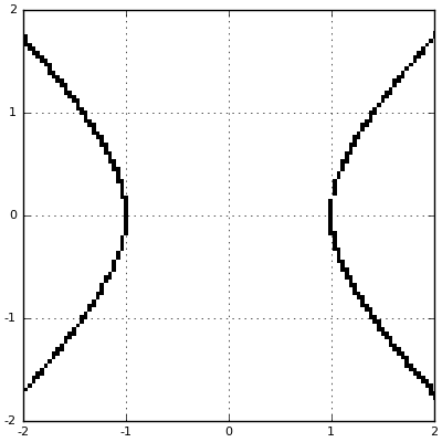
Geometrically, the unit circle on the complex numbers, $\|z\| = 1$, is the familiar unit circle. On the split-complex numbers, the same unit circle is actually a hyperbola. It may not be surprising, then, that the geometry of the split-complex numbers is called a hyperbolic geometry.

An application of the split complex numbers is for (signed) interval arithmetic. Let $a ± b$ be an interval; it represents all numbers in $[a - b, a + b]$. This can be used to represent some kind of physical measurement. If we add two intervals $a ± b$ and $c ± d$, we get the result that $(a + c) ± (b + d)$. You can verify that this is indeed the smallest possible result.

Simultaneously, we note that with split complex numbers,

If we multiply an interval $a ± b$ by a scalar $t$, then the resulting interval should be $ta ± tb$ (presuming that we are working with positive numbers). Multiplying $a ± b$ and $c ± d$ is a little more complicated. Consider the case where $a>b>0$ and $c>d>0$ first. Then we have that $(a-b)(c-d)$ is the smallest possible value, and $(a+b)(c+d)$ is the largest possible value. The midpoint of these is $ac + bd$, and the radius is $ad + bc$.

Simultaneously, we note that with split complex numbers,

This may seem like needless abstraction, but the use of split-complex numbers allows us to use tools from linear algebra. For instance, note that multiplication and addition alone are sufficient to compute any analytic function. Suppose we wish to find

The Dual Numbers

Let's consider another algebra, this time generated by

and we will denote as

Copying over the definition of the norm for complex numbers, we get the norm for dual numbers. If $z = a + b\mathrm{ɛ} ∈ \mathbf{D}$, then

As with the split complex numbers, there are zero divisors in this algebra; they are exactly the scalar multiples of $\mathrm{ɛ}$. So the dual numbers do not form a field.

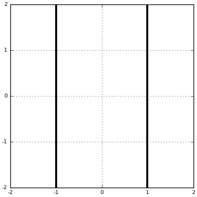
The unit circle $\|z\| = 1$ on the dual numbers is a pair of parallel lines. The geometry of dual numbers is quite strange, because no vertical line segments have any length, and the distance between two points is entirely determined by their horizontal distance. This type of geometry is called a parabolic geometry.

Furthermore, unlike either the complex numbers or the split-complex numbers, the generating element $\mathrm{ɛ}$ of the dual numbers is itself a zero-divisor. Indeed,

Despite these irregularities, the dual numbers are among the most incredible number systems, and are used frequently in computational mathematics. Why? Let $f$ be an analytic function. Then, for any real number $a$, we know that

Define $g(η) = f(a + η)$ which is also analytic, and hence can be extended to the matrices. We now have the remarkable identity:

from which we derive the following corollary, which is the specific case when $b = 1$:

This result means that every analytic function can have its derivative evaluated exactly, which is incredibly useful for many tasks of computational mathematics, optimization, and machine learning.

As an example, let's do a quick problem: Find the derivative of $x^x$. This function is analytic on $(1, ∞)$, so we can use dual numbers. We compute

and extracting the $ɛ$ term,

where every step we took is entirely mechanical and could be done by a computer.

Uniqueness of Hypercomplex Numbers

Above we looked at three distinct kinds of hypercomplex number systems. But are they the only kinds? The answer is that they are, up to isomorphism.

Theorem

Let $A$ be a two-dimensional unital commutative associative $\mathbf{R}$-algebra. Then $A$ is isomorphic to $\mathbf{C}$, or it is isomorphic to $\mathbf{S}$, or it is isomorphic to $\mathbf{D}$.

Proof. Let $1$ be the multiplicative identity, and let $x∈A$ be any vector not parallel to $1$. Then $\operatorname{span}\{1, x\}$ forms a basis. Let $x^2 = a + bx$. We write

Now consider three cases. If $a + \frac{b}{4} = 0$, then $x - \frac{b}{2}$ squares to zero, and since it is not real (since $x$ is not real), therefore $\{1, x - \frac{b}{2}\}$ is a basis. But then $A$ is isomorphic to $\mathbf{D}$.

If $a + \frac{b}{4} < 0$, then

and by a similar argument as before, $A$ is isomorphic to $\mathbf{C}$.

Otherwise, $a + \frac{b}{4} > 0$, and

and hence $A$ is isomorphic to $\mathbf{S}$. QED.